This article introduces Quantum Computing Benchmarking and Certification.
Although still noisy and prone to error, quantum computers are developing at a rapid pace. The field of benchmarking looks at establishing techniques to compare QPU performance in this continuously evolving landscape. Here we highlight some of the topics typically featured in benchmarking research; firstly looking into hardware aspects and qubit characterization, building quantum circuits and the errors encountered at the gate level and finally we highlight some of the techniques involved in certifying performance through algorithm deployment.
For a more detailed assessment of Quantum Computing Benchmarking, including detailed diagrams please contact us.
Importance of quantum computing benchmarking and certification for near term application
Although large scale universal quantum computers have not yet been realized, the current generation of technologies are reaching a point of maturity that is valuable for application. This has seen increased adoption and wider spread access to quantum processing units (QPUs). At a high level, all gate based QPUs operate in a similar way; qubits leverage quantum superposition and entanglement to define gate operations and ultimately logic processing.
A big distinction between such gate based QPUs is that they are based on an exceptionally diverse range of hardware platforms. Furthermore, these technologies are evolving at a rapid pace, with improvements in qubit count, quality, and overall logic processing capacity regularly being announced. This increase in public access along with constant evolution of performance metrics across such a diverse range of technologies ensures the necessity of having benchmarking and certification processes for users to validate the operation of such QPUs.
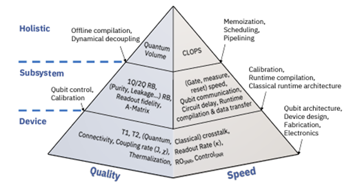
Due to the complex nature of this technology, there are many different points along the QPU stack that are linked to the performance; properties and quality of individual qubits, the quantum circuits that can be constructed from these qubits and finally the interfacing of quantum plane to classical control readout systems and finally the algorithm performance. This means that to compare QPU performance several aspects of the QPU stack and information processing workflow need to be considered

Comparing quantum systems at the individual qubit level:
Qubit number, logic vs physical qubits
Currently one of the most prominent comparison metrics quoted in literature is the qubit number. The thinking here is that the higher the number of qubits, the more powerful the QPU, as it can process larger or more intricate algorithms. On face value this is true, however the reality is much more complex. As the current generation of QPUs still lack rigorous error correction, they are noisy and lead to higher than ideal error rates. One of the ways of dealing with this problem is by encoding the collective quantum state of many individual or ‘physical’ qubits together to form a logical qubit. It is these logical qubits that would be capable of expressing the logic operations defined in a quantum algorithm. So, also it is true that larger number of physical qubits are valuable, as this would relate to a higher number of logical qubits, it is obvious that the number of physical qubits needed to produce a single logical qubit is ultimately related to the quality of the physical qubits. So, it’s more about the balance between qubit quality and number when comparing quantum systems.
Coherence times to gate operation ratio
Qubits, just like any other quantum element are sensitive to their environment. Interaction with the environment can cause decoherence of the quantum state. This means that the qubits have specific time frames or lifetimes during which they are viable for logic processing. This means that to operate the qubit for information processing, control signals or pulses that define the gates, need to be applied to the qubit within the time the quantum state is initiated until it decoheres. Therefore, any series of logic control operation that is conducted on the qubits during algorithm deployment needs to be short enough to fit within this time frame. This time frame is set by two specific time scales:
- The relaxation rate: defined by the time it takes the qubit to spontaneously evolve from an excited state to the ground state. Often called T1.
- The coherence time is the duration the frequency of the qubit is well defined, called T2.
The coherence and relaxation times are key parameters where different qubit technologies vary greatly. For example, superconducting technologies generally have coherence times in the microseconds (μs) whereas optical systems such as the trapped ions can have significantly larger coherence times, into seconds and sometimes even minutes.
As these times scale have a direct impact on the capabilities of the QPU they can serve as a useful metric when comparing technologies. However, it should be noted that speed at which a QPU can operate is ultimately linked to the speed of the gate operations. How many pulses can be applied to the qubits during the coherence time. So, although optical systems may have a much higher coherence time, the pulse widths and are also longer, meaning that the ratio of qubit coherence to gate application times may not be more impressive than superconducting or semiconducting systems with pulses in nanoseconds (ns) time frame.
Single Qubit and Gate Fidelity
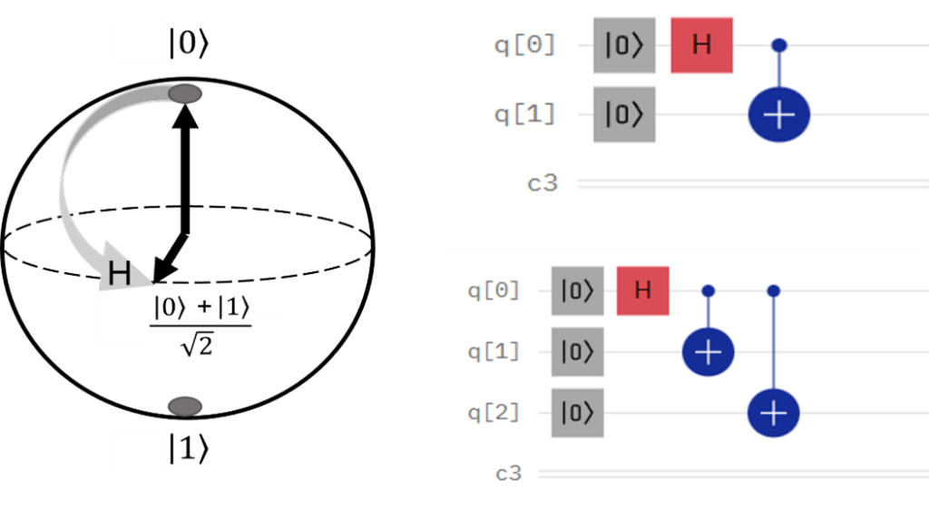
Qubit fidelity is one of the most important metrics that relate qubit quality to performance: Strictly speaking the fidelity, expressed as a percentage, is the probability that a qubit will be in a certain known quantum state after a specific gate operation. In terms of the Bloch sphere, the fidelity gives an idea of the distance between the ideal and actual quantum state after a gate operation/rotation. Knowing the fidelity of individual qubits helps to define error rates as well as possible mechanisms involved in the qubit decoherence. Subsequently, these error rates are related to how noisy the QPU is and how many physical qubits are needed to produce a logical qubit. In general, acceptable single qubit fidelities are above 99%. The single qubit fidelity is typically readily provided by the respective QPU providers.
The fidelity metric is not only applied to individual qubits but also to multiple entangled logic gates. Typically, quantum circuit performance is determined by two qubit gate fidelities. We specifically look at two qubits because this is the smallest number of qubits that can be used to check entanglement. As entanglement is one of the corner stones of quantum computing, the gates involved in entangling qubits are important for benchmarking and performance checks. We call this type of characterization Clifford-gate benchmarking as it involves Clifford algebra, the underlying branch of mathematics that relates quantum mechanics to the information processing operations encoded in the states of qubits (think about the rotations on the block sphere). There is only a hand full of root gates that can be applied to qubits (CNOT, Hadamard, etc.) and all higher order algorithms are built up of these. It makes sense then that two and three qubits gate fidelities are used as comparison metrics as these gates will ultimately influence the operation of larger circuits and algorithms at higher levels of information processing.
Quantum Circuit metrics
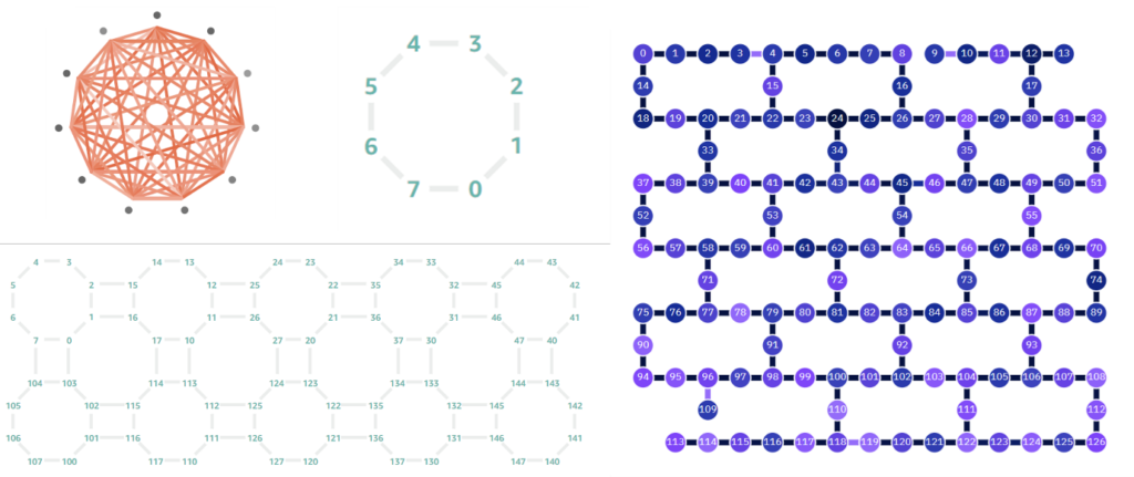
Topology, qubit connectivity
The algorithms used for quantum computing involve leveraging the quantum physics defining the qubit. One of most important aspects of this is entanglement, where the qubits although spatially separated, have a shared state, i.e the control or measurement of the state of one qubit will directly influence another entangled qubit. The gates used in information processing typically involve specific two and three qubit entanglement. The experimental realization of the entanglement is linked to the geometric arrangement of the qubits and the types of connecting pathways that are used to perform the entanglement. A term frequently used to describe this property of the QPU is the connectivity or topology, this parameter essential tell how well qubits are connected or how many qubits other qubits each individual qubit can be entangled with.
This parameter is intimately linked to the type of quantum computer and does show a marked different between modalities. For example, solid state devices such as the supercomputing circuits and the semiconducting qubits are limited by the electrodes/resonators or connecting paths printed on the circuit boards, there are only so many nearest or next nearest neighbor qubits that can be connected through the electronic channels, this results in solid state technologies generally only having two to three direct neighbors which can be directly entangled. Although it is still possible to connect qubits that are very far apart on a circuit through SWAP gates applied to the connecting intermediate qubits, this increases the circuit depth and overall resources required for the information processing, an obvious disadvantage. This however is less of a problem for the optic systems where qubits are not restricted to a two-dimensional circuit board but are linked by a laser induced potential field. This means that there are little restrictions with regard to the qubits/individual atoms being addressed individually and entangled with each other to perform the gate operations that underline the algorithms and logic processing. These types of QPUs therefore have an all-to-all qubit connectivity and do not require any additional SWAP gates to move information around before entangling qubits.
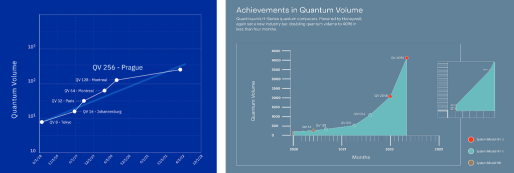
Quantum Volume
Ultimately the capability of a QPU is determined by the size or intricacy of the algorithm it can run (i.e. the problems it can solve). In order to get away from component level metrics related to single qubits, IBM developed an alternative metric in 2018 for evaluating QPU performance: Quantum volume (QV). The quantum volume considers a range of different QPU properties such as qubit number, error rates, cross talk and connectivity. QV is usually expressed as a single value that is empirically measured and not theoretically calculated.
The quantum volume is defined as the size of the largest square circuit that can be successfully run on the processor. This value is obtained by running a circuit that has a depth (longest gate operation sequence in the circuit) equal to its width (number of qubits that define the circuit). Mathematically this is expressed as 2n where n is the circuit depth and width. As an example, a quantum computer that can successfully execute a circuit with depth of 5 on 5 qubits but fails to execute a depth-6 circuit on 6 qubits, would have a quantum volume of 25 or 32. The success of the run is assessed by the probability distribution of the circuit outcome, and usually only distributions with a small statistical deviation are considered successful. Recently modifications to the QV concept have been suggested by IBM where the QV is expressed as a logarithmic scale of QV. Similar redefinition has been suggested by IonQ, where the log of QV was used to Algorithmic qubit. The algorithmic qubit benchmark attempts to move beyond random or trivial gate operations and rather directly looks at the performance of a square circuit composed specifically from gates involving two qubits entanglement (the basis of many higher-level algorithms).
As the QV is dependent on depth, i.e., the sequential flow of gate operations, as well as the width (number of qubits), it inherently helps relate QPU performance to its topology/connectivity, error rates and overall size. Because of this quantum volume is increasingly being used as a QPU performance gauge as it is more holistic and through a single value parameter gives an idea of overall or average performance.
It should also be noted that QV can be somewhat controversial metric as some processors have an inherent advantage due to their underlying hardware. For example, trapped ion systems have an all-to-all- qubit connectivity as well as appreciatively long coherence times, this greatly increases their QV. So, although their operations are generally slower than the high frequency pulsing of superconducting and spin qubits, their QV is reported to be several orders of magnitude higher than their solid-state counterparts.
Circuit Layer Operations per Second (CLOPS)
As mentioned before, different qubits have vastly different relaxation times, coherence times, and gate execution speeds and although they are useful performance metrics, they may not give a true indication of the overall speed at which a QPU can perform its logic processing. This is because the intricacies involved in writing a full program will involve a level of quantum-classical interfacing (only certain tasks are run on the QPU) with algorithms requiring multiple calls to a QPU. Consequently, the runtime system that allows for efficient quantum-classical communication becomes a critical aspect of the information processing and essential to achieving high performance. This runtime interaction has been incorporated into a benchmark metric called Circuit Layer Operations Per Second or CLOPS. CLOPS relies on the definition of QV and gives a measure of how many QV circuits a QPU can execute per unit of time.
Benchmarking and certification practices
Randomized benchmarking:
Quantum State tomography, i.e., the process of measuring and determining the state of the qubits after a set of well-defined gate operations, are in general used to determine the error rates and fidelity of the qubits. Although this is very useful technique, there are some limitations with this. Firstly, it becomes infeasible to apply QST to even moderately sized circuits, and secondly, the very act of conducting a state tomography experiment leads to State-preparation and measurement (SPAM) errors. This means that alternative practices are essential for scaling algorithms on the NISQ devices, especially since these systems are currently expanding at a significant rate.
One practice that has been thoroughly explored is randomized benchmarking. This typically allows for a quantitative characterization of the level of coherent control gate operations. In such protocols one simply measures the exponential decay rate of the fidelity as a function of the length of a random sequence of gates. The measured decay rate is presumed to give an estimate of the average error probability per gate. Therefore, by using RB techniques, it becomes possible to model the error rates of quantum processors. Although already implemented for some time now, this is still an active area of research, with new models to describe the exponential decay and their link to qubit noise still being investigated. As this technique looks directly at noise at the quantum plane, it is a very low-level benchmarking practice, usually focused on the qubit’s performance. Although this is invaluable for enhancing and improving current technologies, it does not give much information on higher level of abstraction on the information processing workflow.
Algorithmic and volumetric benchmarking
Currently state-of-the-art NISQ available are between a few tens to just over one hundred qubits, its becoming increasingly important to look at scalable techniques for benchmarking and especially important for looking at application specific techniques. This need has seen the recent emergence of novel benchmarking practice that evaluates instead of random gates, the performance of specific algorithms that are being explored in the information processing flow. This means that they are more closely related to application and QPU performance tracking for specific tasks. The typical process from in such a practice looks at a volumetric approach to the performance of the QPU for a certain algorithm, i.e. applying quantum volume type processing where the performance is tracked as a function of increasing quantum circuit depth and width.
This means that this type of benchmarking is closely related to algorithm structure and closely linked to quantum circuit properties. This type of benchmarking is at a higher abstraction level compared to randomized techniques, as they are closely related to information processing tasks and not random gate operations. There have already been several instances of application specific benchmarking techniques explored including using VQE for benchmarking in chemistry simulations, through to QAE for monte Carlo sampling. Being based on a volumetric approach, this type of benchmarking is also highly valuable for assessing scalability of NISQ algorithms by tracking algorithm performance as the qubit number of these systems continue to rise.
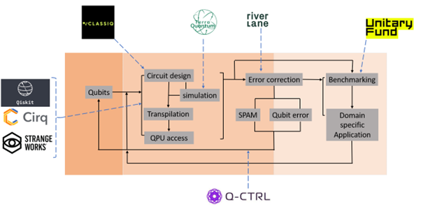
Because of this, it should come as no surprise that the landscape is diverse with several corporations offering solutions or frameworks such as library packages that attempt to tackle the benchmarking problem. Before looking at the benchmarking and certification practices across the software landscape, it is important to understand the workflow in typical quantum logic processing. One the very left initial systems are involved in defining the quantum circuit, things like number of qubits, how the circuit is connected, defining number of shots sent to QPU. Software solutions on this end focus on interfacing with qubits, they provide access to various systems and allow for clear definition or high-level construction of the quantum circuit (based on specific algorithm), after the task gets sent to the hardware provider a step called transpilation occurs, this is an optimization step that maps the virtual quantum circuit to one that is more native to the desired hardware. This is necessary because not every virtually gate can be executed across every type of quantum computer, so transpilation takes the virtual circuit and transforms it into one that would have an (theoretically) identical outcome based on native gates available to a specific QPU. After this task is run, the results can be analyzed. Either a level of error mitigation or feedback control is used to further optimize the algorithm/workflow, or benchmarking is carried out to directly compare results with expected outcomes or other technologies.
As the respective QPU hardware continue to improve, we can undoubtedly expect new techniques for benchmarking and certification. Research in this field is ultimately looking at developing concrete and agreed upon methods similar to those used in classical systems such as the top500 benchmarks. Until a more universal performance gauge is developed, benchmarking remains a very active and exciting space to track.
If you found this article to be informative, you can explore more current quantum news here, exclusives, interviews, and podcasts.