The violation of Bell inequalities has for over fifty years been a challenge to attempts to understand quantum physics. If we can unify our understanding of measurement in classical physics and quantum physics as a Hilbert space analysis of signals we actually measure, as in a previous article here on The Quantum Daily, then we must be able to break or at least weaken the hold of Bell inequalities. Among several ways to do so, we will consider signals that quantum field theory says we could have measured as well as the signals we actually measured. I find it helps to think of a field, classical or quantum, as of measurements and their results, without thinking too much about what the measurements might be of.
John Bell, in “The theory of local beables(PDF)“, says of “The concept of ‘observable′”, that “physically, it is a rather woolly concept”, so he prefers the concept of a ‘beable′. The signal trace we see on an oscilloscope, however, is a rather concrete sequence of many measurement results, actual observations tied to observables, whereas to the contrary whatever might be behind and causing that signal is rather more distant. Thinking about the details of signals instead of only about the singular events that we construct our hardware to identify pushes us away from thinking of a photon as a singular cause of details of the signal, even though we won’t give up trying to imagine whatever better understanding or explanation we might create. A short video of mine from three years ago focuses on events as features of underlying signals:
Before considering the ideas of quantum field theory, we will examine a classic experiment, its raw data, and the analysis of that raw data that gives a violation of the Bell inequalities. We will discipline ourselves not to mention photons whatsoever: everything will be about modulations of statistics of the noisy electromagnetic field contained within the apparatus.
Gregor Weihs’s classic experiment

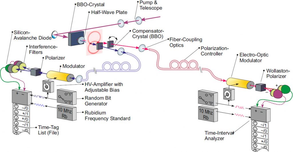
In a crude schematic diagram of an experiment performed by Gregor Weihs just over twenty years ago, described in an article in Physical Review Letters that is included near the end of his PhD thesis(PDF), there are six significant signals, a1, a2, and b1, b2, attached to Alice’s and Bob’s four Avalanche PhotoDiodes (APDs), and A and B, attached to Alice’s and Bob’s ElectroOptic Modulators (EOMs).

A Signal Pump (SP) at the center of the apparatus modulates the electromagnetic field. The apparatus registers very few events in the APDs if the power to the SP is off, so we can say that the SP causes the events that the apparatus starts to register when we turn on the power.
We use exotic materials and electronics when we construct such experiments. Elaborate engineering ensures that the signal in an APD occasionally changes rapidly from zero to a much larger current, then the electronics returns the signal to zero as quickly as possible. The pattern of the A and B signals to the EOMs further modulates the electromagnetic field in the apparatus, which changes the pattern of event timings. Whenever the current in an APD jumps, the apparatus records the time of the event, together with either Alice’s A signal or Bob’s B signal at the time. This is all that Alice and Bob record, but they could instead, for example, measure the six signals every picosecond, allowing more elaborate post-analysis. The SP also uses exotic crystals that have just the right properties for this particular experiment: they’re not just ordinary rocks.
The schematic diagram on Page 60 of Weihs’s thesis gives more sense of the whole apparatus, clearly showing the six signals and the hardware level of the signal analysis:
Visualizing the experimental raw data
To give a first sense of the analysis of the signals, we can graph the timing of every event that Alice registers in one run of the experiment, provided Bob registers an event within three nanoseconds of Alice’s event, over a period of two seconds:

The different symbols denote events in Alice’s two APDs and the two different settings of Alice’s EOM, so there are four possibilities for Alice [and four for Bob: I sadly couldn’t graph all sixteen possibilities legibly.] Alice registers a surplus of events for which Bob registers an almost simultaneous event, close to the horizontal axis. We can zoom out and show all Alice’s events for which Bob registers an event within 200 nanoseconds, over ten seconds, quite randomly distributed except for that middle band of coincident events:
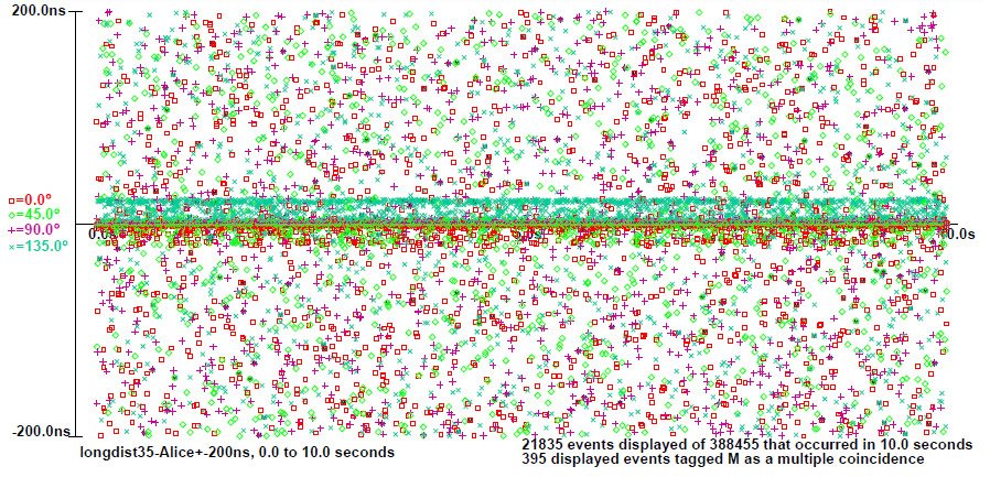
You can find more details of how these graphs were produced here.
The analysis
Everything so far is a perfectly classical record of events that happened during one run of the experiment. It is a compressed record of the six signals a1, a2, b1, b2, A and B. The analysis of the data, however, collects all pairs of simultaneous events into just sixteen different lists. We can see for each of the 16 types of events that there is a clear pattern of diagonal stripes for event pairs that have a separation of less than 3 nanoseconds:

The computed number on the right, 2.714, breaks a Bell inequality because it is greater than 2. The analysis has removed all timing information and has split the APD data into four parts according to the EOM data. That introduces measurement incompatibility, and the breaking of Bell inequalities, for any signal analysis, quantum or classical, because the A signal (and also the B signal) cannot be recorded as two different values at the same time.
What does Quantum Field Theory say?
Suppose we actually recorded the six signals every picosecond instead of only the times of events. This would give us trillions of compatible measurements every second. We would have more information about what happens between the events and about the SP.
A state of a quantum field tells us all the expected statistics of the results for very many compatible measurements that we could record between the measurement results we actually recorded: it fills in what we expect in the gaps at all scales. We can introduce a whole field of such measurements, all across time and space. Such a field can be said to be classical because all the measurements are compatible: in quantum computing they are called quantum non-demolition measurements. They are very difficult but in theory possible to implement. When we consider small enough scales they are so difficult to measure that they are essentially hidden from us.
Even though they come from quantum field theory, such hidden measurements are classical in the sense that they are compatible. The signal analysis of the actual measurement results violates the same Bell inequality, so the statistics of these classical hidden measurements do not satisfy all the conditions that Bell insists they must. If we could perform such hidden measurements, we would find them not to satisfy some of Bell’s conditions. For practical purposes it doesn’t matter how Bell’s statistical conditions are not satisfied, though we could invoke both nonlocality and various statistical dependencies, it only matters that the analysis of actual measurement results breaks Bell inequalities.
Coda
Quantum mechanics has somewhat taken away an idea of what happens between what we measure. We can restore that idea by thinking firstly about actual signals as a sequence of results of compatible measurements instead of only about isolated events, and secondly about other measurements that would have been compatible with those we actually performed.
Until very recently, extensive use of compatible measurements would have seemed a preposterous suggestion. Recall, however, that a previous TQD article shows that “collapse” of the physical state, ρ↦ρZ after a measurement Z, is equivalent to “no-collapse” of the physical state and the use of compatible measurements, X↦XZ, where Z and XZ are compatible: ρZ(X) = ρ(XZ). Quantum field theory gives us a whole field of compatible measurements all the way down to arbitrarily small scales and all across time and space, together with the expected statistics for every combination of such measurements.
The published version of the article in Annals of Physics that underlies the above may be found here [which allows a free download until April 2nd]. A preprint that is fairly close to the published version may be found here. A subsection there suggests that we should investigate exactly how signals change over time in an experiment that violates Bell inequalities immediately after we turn on the power, which is a fundamental thing to know. It’s also a practical thing to know, because sometimes we have power cuts.


